Notation
We will use all the elements of the popular grouped-query attention, with the following variable names:- B batch size
- T sequence length (number of queries)
- S context length (number of keys and values)
- K number of kv heads
- G number of query heads per kv head
- H per-head dimension
What is wrong with naive attention?
Let's start with the simplest version of grouped-query attention. I am using some slightly ugly, low-level ops for the matmuls because these are the ones we will need to write a kernel. This will make sure we always have the same dtype conversions and our numerical checks later will be as precise as possible. I will also assume that queries are already pre-scaled by the usual \(H^{-1/2}\):@jax.jit
def attn_naive(q, k, v):
b, kvh, g, t, h = q.shape
_, _, s, _ = k.shape
assert k.shape == (b, kvh, s, h)
assert v.shape == k.shape
# jnp.einsum('bkgth,bksh->bkgts', q, k)
l = jax.lax.dot_general(
q.astype(jnp.bfloat16),
k.astype(jnp.bfloat16),
(((4,), (3,)), ((0, 1), (0, 1))),
preferred_element_type=jnp.float32,
)
w = jax.nn.softmax(l, axis=-1)
# jnp.einsum('bkgts,bksh->bkgth', w, v)
o = jax.lax.dot_general(
w.astype(jnp.bfloat16),
v.astype(jnp.bfloat16),
(((4,), (2,)), ((0, 1), (0, 1))),
preferred_element_type=jnp.float32,
)
return o.astype(q.dtype)To see why, the key idea is to look at a concept called arithmetic intensity. The How To Scale Your Model book written by my awesome friends and colleagues is an excellent introduction to this topic that I recommend reading first if arithmetic intensity is a new concept to you. To summarize, though:
- The accelerator (which throughout this note is a TPU v6e) is capable of a peak bf16 FLOPS/s \(f_{v6e} = 9.2 \times 10^{14}\) in the matrix multiplication units. Both GPUs and TPUs have dedicated units at the hardware level to deal with matmuls, and note that the peak FLOPS/s often depends on the dtype, e.g., float32 will be slower, and smaller precision dtypes may be faster if the hardware supports it.
- A matmul
ab,b->acentails roughly2abcFLOPS. - In a TPU, to execute a matmul we load the inputs from HBM to VMEM, compute the result into a VMEM buffer, and then move the result from VMEM to HBM. So in bf16 (2 bytes per scalar), our payload for HBM<->VMEM transfers is
2(ab+bc+ca). The TPU v6e has a peak HBM<->VMEM bandwidth bytes/s \(b_{v6e}=1.64\times 10^{12}\). - Combining everything above, this means that for a matmul, we spend \(t_{math} = 2abc/f_{v6e}\) seconds doing math and \(t_{comms} = 2(ab+bc+ca)/b_{v6e}\) seconds in memory transfers. Assuming that our compiler will make sure to overlap byte transfers with math as much as possible, then the total time spent will be \(t=\max(t_{math},t_{comms})\). Now, \(t_{math} > t_{comms} \iff abc/(ab+bc+ca) > f_{v6e}/b_{v6e}\). These ratios in FLOPS/byte are what we call arithmetic intensity, where the LHS \(abc/(ab+bc+ca)\) is the intensity of the matmul, and the RHS \(i_{v6e} = f_{v6e}/b_{v6e} \approx 561\) is the peak intensity of the accelerator (a constant). Generally speaking, we will be compute-bound when the arithemtic intensity of the operation is bigger than \(i_{v6e}\).
Back to attention and arithmetic intensity. In attention, the bulk of the computation lies in the matmuls-- things like softmax and so on are asymptotically negligible. In our naive version, both matmuls have the same arithmetic intensity, each is \(GTHS/(GTH+SH+GTS)\). To see it, just follow the shapes of the inputs and output buffers and it should be trivial to count.
Normally \(G\) (number of query heads divided by the number of kv heads) is very small, \(G=4\) is a common and reasonable choice in modern transformers, so let's use that. And normally \(H\) (the per-head dimension) is a small constant like \(H=128\); to scale the model it is common practice to just use more attention heads, and both \(G\) and \(H\) are kept constant. With these assumptions in place, the intensity during training (i.e., \(T=S\)) will be \(128T/(160+T)\). With some algebra you can work out that this expression will never exceed 128:
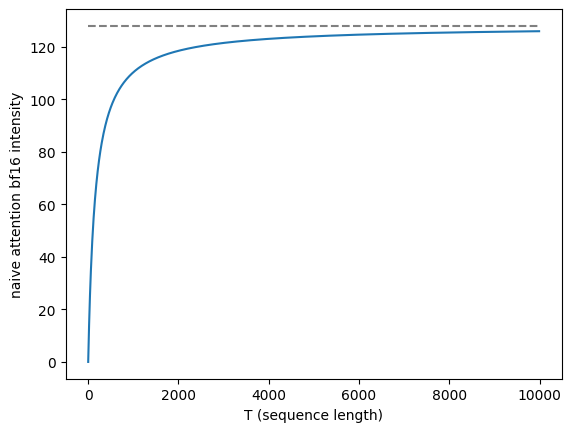
This is bad, because we need the intensity to be larger to be compute bound (e.g., at least 241 on TPU v5e, or at least 561 on TPU v6e), and even though increasing the sequence length increases the intensity, it will never be enough to get us there. In other words, we are starving our chips of compute!
Let's see the running time in practice compared to our estimates using the fact that we will be byte-loading bound, i.e., \(t_{naive} = 4BK(GT+S)H/b_{v6e}\) is our theoretical prediction. In practice, it's of course no better. Here is a measurement of our initial code for different sequence lengths, each instrumented 1024 times and I report the average on a TPU v6e.
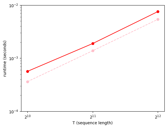
Note though, that if we didn't have the term in the denominator of the intensity \(GTHS/(GTH+SH+GTS)\) that scales as \(O(TS)\), the intensity would grow instead as \(GTS/(GT+S)\), so for training (i.e., \(T=S\)) it would scale unboundedly as \(GT/(G+1)\). In practice, skipping such a term translates to the following question: can we write the computation in a way where we completely avoid HBM<->VMEM transfers for the attention weights? As it turns out, this is exactly what flash attention does!
Quick digression: what about inference? even this strictly better intensity \(GTS/(GT+S)\) that flash attention achieves, during LLM inference \(S\) is the context length and \(T=1\), so the intensity becomes \(GS/(G+S)\), i.e., never greater than \(G=4\). This remains pretty much an open problem with modern LLMs; even with flash attention, autoregressive inference starves AI chips. This chapter in the scaling book talks more in depth about it. You can also see the appeal of things like diffusion models, discrete diffusion, and generally models that train and serve with \(T=S\) or at least \(T\gg 1\): you could do more total FLOPS (e.g., multiple denoising steps) and still be faster than autoregressive inference!
Chunked attention
The first order of business is to talk about VMEM. Unlike HBM, which has many gigabytes worth of space (e.g., 32GB in a TPU v6e), VMEM is a much more precious resource (32MB in a TPU v6e, and a measly 16MB in a TPU v5e). If we reach the intensity that we described above, which scales linearly with \(T\), we would need a sequence length bigger than \(T>i_{v6e}(G+1)/G \approx 702\), so rounding to powers of 2 to stay hardware-friendly, we should have \(t\geq 1024\) to be compute-bound on a TPU v6e. But note that single bf16 \(T\times S\) buffer is already 2MB at \(T=S=1024\). If \(T=S=4096\) or more, we would fully exhaust VMEM. Also note that this is for a single batch element and a single kv-head... Modern LLMs have much larger sequence lengths, so it will be critical to somehow "chunk" the computation over the sequence length to be able to fit the attention weights in VMEM and never write them to HBM.If our attention was linear (i.e., we skip the softmax), this would be fairly easy to do: since we reduce over keys and values in the last matmul, all we need is to accumulate the output and loop over chunks of keys and values:
@functools.partial(jax.jit, static_argnames=('bkv',))
def linear_attn_scan_s(q, k, v, *, bkv=1024):
  _, _, s, _ = k.shape

  def body_fun(i, o):
    kb = jax.lax.dynamic_slice_in_dim(k, i * bkv, bkv, axis=2)
    wb = jax.lax.dot_general(
        q.astype(jnp.bfloat16),
        kb.astype(jnp.bfloat16),
        (((4,), (3,)), ((0, 1), (0, 1))),
        preferred_element_type=jnp.float32,
    )
    vb = jax.lax.dynamic_slice_in_dim(v, i * bkv, bkv, axis=2)
    o += jax.lax.dot_general(
        wb.astype(jnp.bfloat16),
        vb.astype(jnp.bfloat16),
        (((4,), (2,)), ((0, 1), (0, 1))),
        preferred_element_type=jnp.float32,
    )
    return o

  init_val = jnp.zeros(q.shape, dtype=jnp.float32)
return jax.lax.fori_loop(0, s // bkv, body_fun, init_val).astype(q.dtype)1e-5), now we just need to adjust things a bit to re-introduce the softmax. The numerators just go through an element-wise exp which is trivial, but the denominator is trickier because it depends on the entire s-axis. So our strategy will be to accumulate the denominator too-- it is actually a sum over the s-axis. And at the very end we apply the division.
@functools.partial(jax.jit, static_argnames=('bkv',))
def attn_scan_s(q, k, v, *, bkv=1024):
  b, kvh, g, t, h = q.shape
  _, _, s, _ = k.shape
  assert k.shape == (b, kvh, s, h)
  assert v.shape == k.shape
  assert s % bkv == 0

  def body_fun(i, val):
    o, denom = val
    kb = jax.lax.dynamic_slice_in_dim(k, i * bkv, bkv, axis=2)
    lb = jax.lax.dot_general(
        q.astype(jnp.bfloat16),
        kb.astype(jnp.bfloat16),
        (((4,), (3,)), ((0, 1), (0, 1))),
        preferred_element_type=jnp.float32,
    )
    wb = jnp.exp(lb)
    denom += wb.sum(axis=-1)
    vb = jax.lax.dynamic_slice_in_dim(v, i * bkv, bkv, axis=2)
    o += jax.lax.dot_general(
        wb.astype(jnp.bfloat16),
        vb.astype(jnp.bfloat16),
        (((4,), (2,)), ((0, 1), (0, 1))),
        preferred_element_type=jnp.float32,
    )
    return o, denom

  o = jnp.zeros(q.shape, dtype=jnp.float32)
  denom = jnp.zeros(q.shape[:-1], dtype=jnp.float32)
  init_val = (o, denom)
  o, denom = jax.lax.fori_loop(0, s // bkv, body_fun, init_val)
return (o / denom[..., None]).astype(q.dtype)wb = jnp.exp(lb). Indeed, if we feed even slightly large inputs, this will easily return nan ☹️
Most softmax implementations, of course including the one in JAX, solve this well-known problem by subtracting the maximum logit, since \(\mathrm{softmax}(l) = \mathrm{softmax}(l + c)\) for all \(c \in \mathbb{R}\). With \(c=\max(l)\)we ensure every call to
exp will be with a non-positive number, which will always produce a result below 1.0 and will thus not explode.
We need to do a similar trick, but now the issue is that we don't have access to the global maximum since we have chunked things up along the s-axis. Luckily this isn't too bad; we just need to keep a running maximum of the logits and make sure both the numerator and denominator are not scaled by different constants from the maximum subtraction (only when we divide they cancel out):
@functools.partial(jax.jit, static_argnames=('bkv',))
def attn_scan_s_stable(q, k, v, *, bkv=1024):
  b, kvh, g, t, h = q.shape
  _, _, s, _ = k.shape
  assert k.shape == (b, kvh, s, h)
  assert v.shape == k.shape
  assert s % bkv == 0

  def body_fun(i, val):
    o, denom, m = val
    kb = jax.lax.dynamic_slice_in_dim(k, i * bkv, bkv, axis=2)
    lb = jax.lax.dot_general(
        q.astype(jnp.bfloat16),
        kb.astype(jnp.bfloat16),
        (((4,), (3,)), ((0, 1), (0, 1))),
        preferred_element_type=jnp.float32,
    )
    m_new = jnp.maximum(m, lb.max(axis=-1))
    corr = jnp.exp(m - m_new)
    wb = jnp.exp(lb - m_new[..., None])
    denom = denom * corr + wb.sum(axis=-1)
    vb = jax.lax.dynamic_slice_in_dim(v, i * bkv, bkv, axis=2)
    o = o * corr[..., None] + jax.lax.dot_general(
        wb.astype(jnp.bfloat16),
        vb.astype(jnp.bfloat16),
        (((4,), (2,)), ((0, 1), (0, 1))),
        preferred_element_type=jnp.float32,
    )
    return o, denom, m_new

  o = jnp.zeros(q.shape, dtype=jnp.float32)
  denom = jnp.zeros(q.shape[:-1], dtype=jnp.float32)
  m = jnp.full(q.shape[:-1], -jnp.inf, dtype=jnp.float32)
  init_val = (o, denom, m)
  o, denom, m = jax.lax.fori_loop(0, s // bkv, body_fun, init_val)
return (o / denom[..., None]).astype(q.dtype)What we have so far: we now have a chunked attention that is numerically stable and very close numerically to the original naive version, even with bf16 matmuls! This is NOT enough to get flash-performance, because even with these smaller matmuls for the attention weights, we are still transferring each of their results from VMEM to HBM and then from HBM to VMEM when we do the matmul with the attention values. Still, now we have full control over the KV chunk sizes. So we can make them big enough to be compute-bound during training, but small enough to not run out of VMEM once we actually eliminate the memory transfers.
What we need: we must now write some lower-level code to ensure each attention weights chunk actually skips such memory transfers.
At this point, it should now be clear why flash attention should both save memory and be faster-- we can fully utilize the accelerator with large enough block sizes, we avoid additional memory transfers, and the attention weights which scale as \(O(TS)\) will never be present in HBM.
Our first kernel
Before we start, let's write our previous function such that it's more clear what exactly we will replace with a kernel. We will also vmap over the batch and kv-heads dimensions so the kernel has to deal with as few dimensions as possible. Nothing functional is changing; this is just a small refactor for better clarity:@functools.partial(jax.jit, static_argnames=('bkv',))
def attn_scan_s_nokernel(q, k, v, *, bkv=1024):
b, kvh, g, t, h = q.shape
_, _, s, _ = k.shape
assert k.shape == (b, kvh, s, h)
assert v.shape == k.shape
assert s % bkv == 0
@jax.vmap # over b
@jax.vmap # over kvh
def kernel(q, kb, vb, o, denom, m):
# --- TODO: optimize!
lb = jax.lax.dot_general(
q.astype(jnp.bfloat16),
kb.astype(jnp.bfloat16),
(((2,), (1,)), ((), ())),
preferred_element_type=jnp.float32,
)
m_new = jnp.maximum(m, lb.max(axis=-1))
corr = jnp.exp(m - m_new)
wb = jnp.exp(lb - m_new[..., None])
denom = denom * corr + wb.sum(axis=-1)
o = o * corr[..., None] + jax.lax.dot_general(
wb.astype(jnp.bfloat16),
vb.astype(jnp.bfloat16),
(((2,), (0,)), ((), ())),
preferred_element_type=jnp.float32,
)
# --- END TODO
return o, denom, m_new
def body_fun(i, val):
o, denom, m = val
kb = jax.lax.dynamic_slice_in_dim(k, i * bkv, bkv, axis=2)
vb = jax.lax.dynamic_slice_in_dim(v, i * bkv, bkv, axis=2)
return kernel(q, kb, vb, o, denom, m)
o = jnp.zeros(q.shape, dtype=jnp.float32)
denom = jnp.zeros(q.shape[:-1], dtype=jnp.float32)
m = jnp.full(q.shape[:-1], -jnp.inf, dtype=jnp.float32)
o, denom, m = jax.lax.fori_loop(0, s // bkv, body_fun, (o, denom, m))
return (o / denom[..., None]).astype(q.dtype)While I can't give a full introduction to Pallas, the key detail that matters most is that functions wrapped with
pallas_call will have arguments corresponding to MemoryRef instances rather than JAX arrays. foo = myref[...] explicitly reads the memory ref, and myref[...] = foo explicitly writes to it.
Unless we configure things differently, the default for a kernel is that those memory refs are pointing to buffers in VMEM. Inside the kernel, the outermost memory we work with is VMEM, and pallas will handle the HBM<->VMEM transfers of the inputs and outputs to the kernel. This way we will make sure the attention logits and weights never leave. Pallas will also handle placement of the intermediates in our program-- if they're very small, they might even stay in VREGs, otherwise VMEM will be used.
The code below may look a bit scary, but it's mostly just setting up the extra VMEM buffers we need, explicitly reading and writing to buffers, and specifying how to tile the kernel into parallel programs. The math is identical to the version above, nothing has changed!
  @jax.vmap  # over b
  @jax.vmap  # over kvh
  @functools.partial(
      pl.pallas_call,
      # The kernel runs t // bq programs. Explicitly chunking the program by
      # queries in the kernel will now also let us control the T-dimension of
      # our block sizes that must fit in VMEM. The keys and values are already
      # chunked by the outer loop.
      grid=(t // bq,),
      # The kernel chunks inputs into blocks with the following sizes
      # and maps each block into the i-th program via each specified map.
      in_specs=(
          pl.BlockSpec((g, bq, h), lambda i: (0, i, 0)),  # q
          pl.BlockSpec((bkv, h), lambda i: (0, 0)),       # kb
          pl.BlockSpec((bkv, h), lambda i: (0, 0)),       # vb
          pl.BlockSpec((g, bq, h), lambda i: (0, i, 0)),  # o
          pl.BlockSpec((g, bq), lambda i: (0, i)),        # d
          pl.BlockSpec((g, bq), lambda i: (0, i)),        # m
      ),
      # The outputs for the i-th program are similarly chunked and the final
      # result in HBM will be re-grouped. Note that it is not allowed to write
      # to input refs, so we must use different refs for the output carries.
      out_specs=(
          pl.BlockSpec((g, bq, h), lambda i: (0, i, 0)),  # oo
          pl.BlockSpec((g, bq), lambda i: (0, i)),        # od
          pl.BlockSpec((g, bq), lambda i: (0, i)),        # om
      ),
      out_shape=(
          jax.ShapeDtypeStruct((g, t, h), jnp.float32),  # oo
          jax.ShapeDtypeStruct((g, t), jnp.float32),     # od
          jax.ShapeDtypeStruct((g, t), jnp.float32),     # om
      ),
      # Since attention is fully parallelizable over queries, we tell pallas
      # that the t // bq programs can run in parallel.
      compiler_params=pltpu.CompilerParams(dimension_semantics=('parallel',)),
  )
  def kernel(
      # --- Inputs.
      qref,
      kbref,
      vbref,
      oref,
      dref,
      mref,
      # --- Outputs.
      ooref,
      odref,
      omref,
  ):
    l = jax.lax.dot_general(
        qref[...].astype(jnp.bfloat16),
        kbref[...].astype(jnp.bfloat16),
        (((2,), (1,)), ((), ())),
        preferred_element_type=jnp.float32,
    )
    m_new = jnp.maximum(mref[...], l.max(axis=-1))
    omref[...] = m_new
    c = jnp.exp(mref[...] - m_new)
    w = jnp.exp(l - m_new[..., None])
    odref[...] = dref[...] * c + w.sum(axis=-1)
    o_new = jax.lax.dot_general(
        w.astype(jnp.bfloat16),
        vbref[...].astype(jnp.bfloat16),
        (((2,), (0,)), ((), ())),
        preferred_element_type=jnp.float32,
    )
ooref[...] = oref[...] * c[..., None] + o_new1e-9. Nice!
Let's check the performance of the kernel now. We need a real baseline, so we try out the splash attention kernel in JAX. The "splash" name stands for sparse flash attention. This kernel has some extra neat tricks to reduce both FLOPS and byteload if there are zeros in the causal mask. In our case, we're working with no masking, i.e., a mask full of ones. You can use this helper function to make a splash function that uses shapes like ours, is also optimized for GQA (i.e., it doesn't tile kv heads which leads to increased byteload), has the same block size conventions, and allows us to jit it ourselves after vmapping it:
from jax.experimental.pallas.ops.tpu.splash_attention import splash_attention_kernel
from jax.experimental.pallas.ops.tpu.splash_attention import splash_attention_mask
from jax.experimental.pallas.ops.tpu.splash_attention import splash_attention_mask_info

def make_splash_fn_nojit(*, t, s, bq=1024, bkv=1024):
  splash_block_sizes = splash_attention_kernel.BlockSizes(
      block_q=bq, block_kv=bkv,
  )
  fwd_mask_info, mask_function_fwd = splash_attention_mask_info.process_mask(
      splash_attention_mask.MultiHeadMask(
          [splash_attention_mask.FullMask((t, s))]
      ),
      (splash_block_sizes.block_q, splash_block_sizes.block_kv),
  )
  f = lambda qq, kk, vv: splash_attention_kernel._splash_attention_custom(
      fwd_mask_info=fwd_mask_info,
      dq_mask_info=None,
      dkv_mask_info=None,
      q=qq,
      k=kk,
      v=vv,
      segment_ids=None,
      sinks=None,
      save_residuals=False,
      mask_value=splash_attention_kernel.DEFAULT_MASK_VALUE,
      is_mqa=True,
      block_sizes=splash_block_sizes,
      residual_checkpoint_name=None,
      mask_function=mask_function_fwd,
  )
return jax.vmap(jax.vmap(f))bq=bkv=1024 should suffice. Our theoretical estimate is now gonna be based in FLOPS: it is \(4BKGTSH/f_{v6e}\).
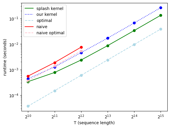
Now we're doing better than vanilla attention could ever do! Also, we can go to pretty long sequence lengths like 32768 on TPU v6e, compared to 4096 which was the last power of 2 that fit in HBM with naive attention. Neat! But we're still quite far from the compute-bound roofline, and a bit worse than the baseline. What else could we do?
Optimizing the kernel
It shouldn't be too surprising that it will be tough to imrove things a lot, since the JAX splash attention baseline is also pretty far from the roofline. There are some easy to see and fix things that can let us push a bit further though!One issue is that we're invoking the kernel many times, reading and writing the
(o, d, m) carries from HBM<->VMEM. Instead, we could make the KV loop part of the kernel and avoid these transfers. For this, we make our kernel a 2D grid of programs and tell Pallas that the KV loop must run sequentially. Pallas also allows us to allocate scratch VMEM that can persist across program invocations, so we can even initialize the carries in VMEM and have them never leave. Another detail is that we should also make sure the kernel output is in bf16 to cut the output byteload by half, even if the scratch buffer for the output carry still accumulates in fp32.
@functools.partial(jax.jit, static_argnames=('bq', 'bkv',))
def flash_attention(q, k, v, *, bq=1024, bkv=1024):
  b, kvh, g, t, h = q.shape
  _, _, s, _ = k.shape
  assert k.shape == (b, kvh, s, h)
  assert v.shape == k.shape
  assert s % bkv == 0
  assert bkv % 128 == 0
  assert t % bq == 0

  @jax.vmap  # over b
  @jax.vmap  # over kvh
  @functools.partial(
      pl.pallas_call,
      grid=(t // bq, s // bkv),
      in_specs=(
          pl.BlockSpec((g, bq, h), lambda i, j: (0, i, 0)),  # q
          pl.BlockSpec((bkv, h), lambda i, j: (j, 0)),       # k
          pl.BlockSpec((bkv, h), lambda i, j: (j, 0)),       # v
      ),
      out_specs=(
          pl.BlockSpec((g, bq, h), lambda i, j: (0, i, 0)),  # o
      ),
      out_shape=(
          jax.ShapeDtypeStruct((g, t, h), q.dtype),          # o (NOW BF16!!!)
      ),
      scratch_shapes=(
          pltpu.VMEM((g, bq, h), jnp.float32),    # acc (o carry)
          pltpu.VMEM((g, bq), jnp.float32),       # denom carry
          pltpu.VMEM((g, bq), jnp.float32),       # m carry
      ),
      compiler_params=pltpu.CompilerParams(
          dimension_semantics=('parallel', 'arbitrary'),
      ),
  )
  def kernel(qref, kref, vref, oref, acc, denom, m):
    j = pl.program_id(1)

    @pl.when(j == 0)
    def _():
      acc[...] = jnp.zeros_like(acc)
      denom[...] = jnp.zeros_like(denom)
      m[...] = jnp.full_like(m, -jnp.inf)

    l = jax.lax.dot_general(
        qref[...].astype(jnp.bfloat16),
        kref[...].astype(jnp.bfloat16),
        (((2,), (1,)), ((), ())),
        preferred_element_type=jnp.float32,
    )
    m_new = jnp.maximum(m[...], l.max(axis=-1))
    c = jnp.exp(m[...] - m_new)
    w = jnp.exp(l - m_new[..., None])
    m[...] = m_new
    denom[...] = denom[...] * c + w.sum(axis=-1)
    o_new = jax.lax.dot_general(
        w.astype(jnp.bfloat16),
        vref[...].astype(jnp.bfloat16),
        (((2,), (0,)), ((), ())),
        preferred_element_type=jnp.float32,
    )
    acc[...] = acc[...] * c[..., None] + o_new

    @pl.when(j == s // bkv - 1)
    def _():
      oref[...] = (acc[...] / denom[...][..., None]).astype(q.dtype)

  o, = kernel(q, k, v)
return obq=bkv=1024 like before:
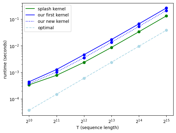
This clearly helped, but it's not the most impactful thing right now-- we need a lot more to outperform the JAX baseline. Still, once we get there, these optimizations will definitely stop being negligible.
One reason why even the baseline struggles to get close to the roofline is that we have a lot going on between the two attention matmuls. Operations like elementwise additions, multiplications,
exp, reductions, all have very low arithmetic intensity. The hardware is fully aware of this and comes with different dedicated cores (on TPUs this is called the VPU, and GPUs have a "warp scheduler" on each streaming multiprocessor) which have lower peak intensity than the matrix cores and take care of such ops. Still, their peak FLOPS/s is nowhere near that of the matrix units. FWIW, the Flash Attention 2 paper reports that the original Flash Attention kernel could only reach 25-40% the speed v.s. that of the compute-bound roofline.
This means that the most impactful thing we could do to improve performance is not chasing the tail of small optimizations in the kernel, but rather tune the block sizes! The key observation is that the number of VPU ops we are doing scales with the number of KV blocks. So we want less, bigger KV blocks. Unfortunately, if we use a bigger \(T\times S\) (i.e., the next power of 2) we will already exhaust VMEM. So one option is to use \(T=512, S=2048\); or \(T=256, S=4096\). In a TPU v6e this is the limit; \(T=128, S=8192) leads to a VMEM OOM. This happens because the input KV blocks grow unboundedly (they do not have a T-axis where we normally perform smaller chunking over to keep the total block size constant).
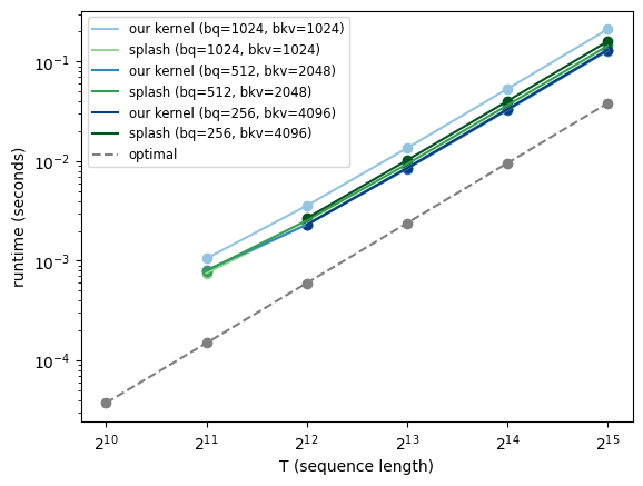
And now things are looking much better for us, and about the same for the splash kernel. The takeaway should be how important it is to tune the block sizes-- devices with more VMEM (e.g., TPU v6e has 2x VMEM than TPU v5e) can fit larger \(T\times S\) chunks, and bigger KV blocks can remove a bunch of VPU ops (though with each increase we use more VMEM and the number of ops pruned is half less than the previous step).